Problem Decomposition

Overview

Teaching: 30 min
Exercises: 0 min

Questions

• How do I structure my data and program to work in parallel?

Objectives

• Understand the main strategies for parallelizing algorithms and data.

• Learn about different decomposition techniques.

• See how decomposition is used on a real problem.

One of the first steps in designing a parallel program is to break the problem into discrete “chunks” of work that can be distributed to multiple tasks so the can work on on the problem simultaneously. This is known as decomposition or partitioning. There are two main ways to decompose an algorithm: domain decomposition and functional decomposition.

Domain decomposition

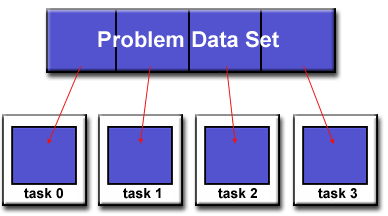
In this type of partitioning, the data associated with a problem is decomposed. Each parallel task then works on a portion of the data.

Key characteristics of domain decomposition are:

• Data divided into pieces of same size and mapped to different processors
• Processor works only on data assigned to it
• Communicates with other processors when necessary

There are many different ways to partition the data.

Examples of domain decomposition

• Embarrassingly parallel applications (Monte Carlo simulations)
• Finite difference calculations
• Numerical integration

Functional decomposition

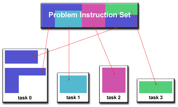
For function decomposition, the focus is on the computation that is to be performed rather than on the data manipulated by the computation. The problem is decomposed according to the work that must be done. Each task then performs a portion of the overall work.

Key characteristics of functional decomposition are:

• Used when pieces of data require different processing times
• Performance limited by the slowest process
• Program decomposed into a number of small tasks
• Tasks assigned to processors as they become available
• Implemented in a master/slave paradigm

Examples of functional decomposition

• Surface reconstruction from a finite element mesh
• Searching images or data bases

Domain decomposition example

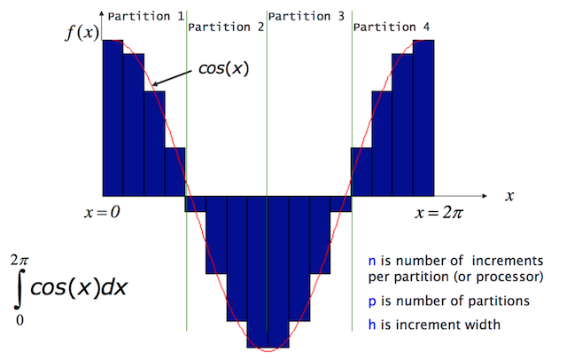
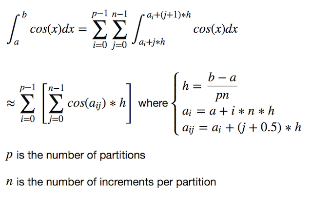
An example of domain decomposition can be seen by computing a simple integral using the Mid-point rule.

Serial version

An example of the serial code to implement this is:

from math import acos, cos

# Compute the inner sum
def integral(a_i, h, n):
    integ = 0.0
    for j in range(n):
        a_ij = a_i + (j + 0.5) * h
        integ += cos(a_ij) * h
    return integ
    
pi = 3.14159265359
p = 4
n = 500
a = 0.0
b = pi / 2.0
h = (b - a) / (n * p)

integral_sum = 0.0

# Compute the outer sum
for i in range(p):
    a_i = a + i * n * h
    integral_sum += integral(a_i, h, n)
    
print("The integral = ", integral_sum)

When run, this code generates the following output:

The integral =  1.0000000257

Parallel point-to-point version

Since the problem has already been decomposed into separate partitions, it is easy to implement a parallel version of the algorithm. In this case, each of the partitions can be computed by a separate process. Once each process has computed its partition, it sends the result back to a root process (in this case process 0) which sums the values and prints the final result.

import numpy
from math import acos, cos
from mpi4py import MPI
comm = MPI.COMM_WORLD
rank = comm.Get_rank()
size = comm.Get_size()

def integral(a_i, h, n):
    integ = 0.0
    for j in range(n):
        a_ij = a_i + (j + 0.5) * h
        integ += cos(a_ij) * h
    return integ

pi = 3.14159265359
n = 500
a = 0.0
b = pi / 2.0
h = (b - a) / (n * size)
a_i = a + rank * n * h

# All processes initialize my_int with their partition calculation
my_int = numpy.full(1, integral(a_i, h, n))

print("Process ", rank, " has the partial integral ", my_int[0])

if rank == 0:
    # Process 0 receives all the partitions and computes the sum
    integral_sum = my_int[0]
    for p in range(1, size):
        comm.Recv(my_int, source=p)
        integral_sum += my_int[0]

    print("The integral = ", integral_sum)
else:
    # All other processes just send their partition values to process 0
    comm.Send(my_int, dest=0)

This program can be run with the following command:

mpiexec -n 4 python midpoint_par.py

When run, output similar to the following will be generated:

Process  0  has the partial integral  0.382683442201
The integral =  1.0000000257
Process  1  has the partial integral  0.32442335716
Process  2  has the partial integral  0.216772756896
Process  3  has the partial integral  0.0761204694451

Key Points

• Domain decomposition is how data is partitioned.

• Functional decomposition is how an algorithm is partitioned.

• Some problems are better suited to one type of decomposition than others.